from pandas.plotting import register_matplotlib_converters

register_matplotlib_converters()

import warnings

warnings.filterwarnings("ignore")
Data Access#
servers, servers everywhere and not a bit to flip#

whoami#
ocefpaf (Filipe Fernandes)
Physical Oceanographer
Data Plumber
Code Janitor
CI babysitter
Amazon-Dash-Button for conda-forge
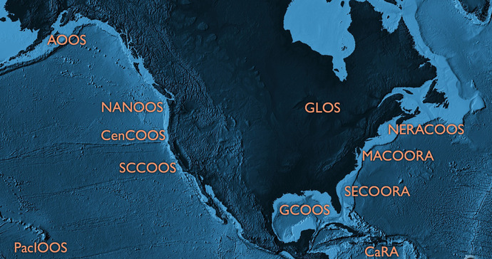
My day job: IOOS#

Big or small we need data!#
There are various sources: variety of servers, APIs, and web services. Just to list a few: OPeNDAP, ERDDAP, THREDDS, ftp, http(s), S3, LAS, etc.

Feedback#
As you suffer from my tutorial on Data Access I’d love that you keep the following questions in mind so we can improve the tutorials. Should this tutorial focus on?
Leveraging metadata for finding data and exploring data?
Software packages to access, slice, and dice data?
Data sources?
None of the above, we don’t need this tutorial!
Web Services/Type of servers#
Data Type |
Web Service |
Response |
|---|---|---|
In-situ data |
OGC SOS |
XML/CSV |
Gridded data (models, satellite) |
OPeNDAP |
Binary |
Raster Images |
OGC WMS |
GeoTIFF/PNG |
ERDDAP |
Restful API |
* |
Your imagination is the limit!
What are we going to see in this tutorial?#
Browse and access data from:
ERDDAP
OPeNDAP
~~SOS~~
WMS
CSW and CKAN*
* There are many examples on CSW in [the IOOS code lab] jupyter-book (https://ioos.github.io/ioos_code_lab/content/intro.html).
1) ERDDAP#
Learning objectives:#
Explore an ERDDAP server with the python interface (erddapy);
Find a data for a time/region of interest;
Download the data with a familiar format and create some plots.
What is ERDDAP?#
Flexible outputs: .html table, ESRI .asc and .csv, .csvp, Google Earth .kml, OPeNDAP binary, .mat, .nc, ODV .txt, .tsv, .json, and .xhtml
RESTful API to access the data
Standardize dates and time in the results
Server-side searching and slicing
from erddapy import ERDDAP

server = "http://erddap.dataexplorer.oceanobservatories.org/erddap"

e = ERDDAP(server=server, protocol="tabledap")
What services are available in the server?#
import pandas as pd

df = pd.read_csv(
    e.get_search_url(
        response="csv",
        search_for="all",
    )
)
print(
    f'We have {len(set(df["tabledap"].dropna()))} '
    f'tabledap, {len(set(df["griddap"].dropna()))} '
    f'griddap, and {len(set(df["wms"].dropna()))} wms.'
)
Let’s query all the datasets that have the standard_name of sea_water_practical_salinity.#
url = e.get_categorize_url(
    categorize_by="standard_name",
    value="sea_water_practical_salinity",
    response="csv",
)

df = pd.read_csv(url)
dataset_ids = df.loc[~df["tabledap"].isnull(), "Dataset ID"].tolist()

dataset_ids_list = "\n".join(dataset_ids)
print(f"Found {len(dataset_ids)} datasets")
Let us narrow our search to deployments that within a lon/lat/time extent.#
from ipyleaflet import FullScreenControl, Map, Rectangle

min_lon, max_lon = -72, -69
min_lat, max_lat = 38, 41

rectangle = Rectangle(bounds=((min_lat, min_lon), (max_lat, max_lon)))

m = Map(
    center=((min_lat + max_lat) / 2, (min_lon + max_lon) / 2),
    zoom=6,
)

m.add_layer(rectangle)
m.add_control(FullScreenControl())
m
kw = {
    "min_time": "2016-07-10T00:00:00Z",
    "max_time": "2017-02-10T00:00:00Z",
    "min_lon": min_lon,
    "max_lon": max_lon,
    "min_lat": min_lat,
    "max_lat": max_lat,
    "standard_name": "sea_water_practical_salinity",
}
search_url = e.get_search_url(response="csv", **kw)
search = pd.read_csv(search_url)
dataset_ids = search["Dataset ID"].values

dataset_ids_list = "\n".join(dataset_ids)
print(f"Found {len(dataset_ids)} Datasets:\n{dataset_ids_list}")
sal = "sea_water_practical_salinity_profiler_depth_enabled"
temp = "sea_water_temperature_profiler_depth_enabled"

e.dataset_id = dataset_ids[0]

e.variables = [
    "z",
    "latitude",
    "longitude",
    sal,
    temp,
    "time",
]

url = e.get_download_url()
print(url)
import pandas as pd

df = e.to_pandas(index_col="time (UTC)", parse_dates=True).dropna()

df.head()
Exercise: experiment with the e.to_xarray() method. Think about why/where use
one or the other?
import matplotlib.pyplot as plt

subset = df.loc[df["z (m)"] == df["z (m)"].min()]

fig, ax = plt.subplots(figsize=(13, 3.75))
subset[f"{sal} (1e-3)"]["2016"].dropna().plot(ax=ax)
import gsw
import numpy as np


def plot_ts():
    fig, ax = plt.subplots(figsize=(5, 5))

    s = np.linspace(0, 42, 100)
    t = np.linspace(-2, 40, 100)

    s, t = np.meshgrid(s, t)
    sigma = gsw.sigma0(s, t)

    cnt = np.arange(-7, 40, 5)
    cs = ax.contour(s, t, sigma, colors="gray", levels=cnt)
    ax.clabel(cs, fontsize=9, inline=1, fmt="%2i")

    ax.set_xlabel("Salinity [g kg$^{-1}$]")
    ax.set_ylabel("Temperature [$^{\circ}$C]")
    ax.scatter(df[f"{sal} (1e-3)"], df[f"{temp} (degree_Celsius)"], s=10, alpha=0.25)

    ax.grid(True)
    ax.axis([20, 40, 4, 26])
    return fig, ax
fig, ax = plot_ts()
responses = ["mat", "json", "ncCF", "ncCFHeader"]

for response in responses:
    print(f"{e.get_download_url(response=response)}\n")
Exercise: explore the web interface for the OOI server URL:
http://erddap.dataexplorer.oceanobservatories.org/erddap/index.html
or the IOOS glider dac:
https://gliders.ioos.us/erddap
and find a dataset of interested, download a format that you are familiar with and plot it (using the web interface or the Python, your choice).
2) OPeNDAP#
Learning objectives:#
Open model data from a THREDDS server via OPeNDAP with
xarray;Discuss the differences with an
erddapyrequest;Plot it using
xarrayinterface.
import cf_xarray
import xarray as xr

url = (
    "http://tds.marine.rutgers.edu/thredds/dodsC/roms/doppio/2017_da/avg/Averages_Best"
)
ds = xr.open_dataset(url)
ds.cf
variable = "sea_water_potential_temperature"
time = "2022-08-10"
surface = -1

selection = ds.cf[variable].sel(time="2022-08-10").isel(s_rho=surface)
import cartopy.crs as ccrs
import matplotlib.pyplot as plt

fig, ax = plt.subplots(
    figsize=(6, 6),
    subplot_kw={"projection": ccrs.PlateCarree()},
)

selection.plot(
    ax=ax,
    x="lon_rho",
    y="lat_rho",
)

ax.coastlines()
3) ~~SOS~~#
Learning objectives:#
Use searvey to obtain CO-OPS data
import shapely
from searvey import coops

secoora = shapely.geometry.box(-87.4, 24.25, -74.7, 36.7)
df = coops.coops_stations_within_region(secoora)
df
df.loc[df["name"] == "Duck"]
from datetime import datetime, timedelta

from searvey.coops import COOPS_Station

station = COOPS_Station("Duck")

ds = station.product(
    "water_level",
    start_date=datetime.today() - timedelta(15),
    end_date=datetime.today(),
)

ds["v"].plot()
4) WMS#
Learning objectives:#
Add a WMS layer to an interactive map. (“Hurricane viz widget.”)
from ipyleaflet import FullScreenControl, Map, WMSLayer, basemaps
from ipywidgets import SelectionSlider
from traitlets import Unicode

time_options = [
    "13:00",
    "13:30",
    "14:00",
    "14:30",
    "15:00",
    "15:30",
    "16:00",
    "16:30",
    "17:00",
    "17:30",
    "18:00",
    "18:30",
]

slider = SelectionSlider(description="Time:", options=time_options)


def update_wms(change):
    time_wms.time = "2020-07-25T{}".format(slider.value)


slider.observe(update_wms, "value")


class TimeWMSLayer(WMSLayer):
    time = Unicode("").tag(sync=True, o=True)
time_wms = TimeWMSLayer(
    url="https://mesonet.agron.iastate.edu/cgi-bin/wms/nexrad/n0r-t.cgi?",
    layers="nexrad-n0r-wmst",
    time="2020-07-25T13:00:00Z",
    format="image/png",
    transparent=True,
    attribution="Weather data © 2012 IEM Nexrad",
)
m = Map(basemap=basemaps.CartoDB.Positron, center=(30, -88), zoom=5)
m.add_layer(time_wms)
m.add_control(FullScreenControl())
m
slider
5) Catalog Service Web (CSW)#
Is there a canonical source for data?#

Well, kind of… The closet thing is are data catalogs like the IOOS CSW catalog or pangeo-forge.
Catalog Service for the Web (CSW)#
A single source to find endpoints
Nice python interface:
owslib.csw.CatalogueServiceWebAdvanced filtering:
owslib.fes
For more complex examples on how to find data in the catalog please check the IOOS code gallery:#
Where to find data?#
Curated list of ERDDAP servers: https://github.com/IrishMarineInstitute/awesome-erddap
Environmental Data Service (EDS) model viewer: https://eds.ioos.us
Exploring THREDDS servers: https://unidata.github.io/siphon/latest
Extras: how does this all work?#
Standards!#

Bad example#
import cftime
import nc_time_axis
from netCDF4 import Dataset

url = "http://goosbrasil.org:8080/pirata/B19s34w.nc"
nc = Dataset(url)

temp = nc["temperature"][:]
times = nc["time"]
temp[temp <= -9999] = np.NaN
t = cftime.num2date(times[:], times.units, calendar=times.calendar)
mask = (t >= datetime(2008, 1, 1)) & (t <= datetime(2008, 12, 31))
fig, ax = plt.subplots()
ax.plot(t[mask], temp[:, 0][mask], ".")
Good example#
import xarray as xr

ds = xr.open_dataset(url)
temp = ds["temperature"]
temp.sel(depth_t=1.0, time="2008").plot()

